Basic Exploratory Data Analysis and Simple Linear Regression in Python
Using pandas, matplot, and seaborn library.
 Image credit: Kim Ellis
Import Library
import math
import pandas as pd
import matplotlib.pyplot as plt
import seaborn as sns
from sklearn.linear_model import LinearRegression

# Visulaization options:
%matplotlib inline
Read data
Data obtained from UCI Machine Learning Repository & accessed via Kaggle (https://www.kaggle.com/uciml/red-wine-quality-cortez-et-al-2009)
df = pd.read_csv("redwine.csv")
df
| fixed acidity | volatile acidity | citric acid | residual sugar | chlorides | free sulfur dioxide | total sulfur dioxide | density | pH | sulphates | alcohol | quality | |
|---|---|---|---|---|---|---|---|---|---|---|---|---|
| 0 | 7.4 | 0.700 | 0.00 | 1.9 | 0.076 | 11.0 | 34.0 | 0.99780 | 3.51 | 0.56 | 9.4 | 5 |
| 1 | 7.8 | 0.880 | 0.00 | 2.6 | 0.098 | 25.0 | 67.0 | 0.99680 | 3.20 | 0.68 | 9.8 | 5 |
| 2 | 7.8 | 0.760 | 0.04 | 2.3 | 0.092 | 15.0 | 54.0 | 0.99700 | 3.26 | 0.65 | 9.8 | 5 |
| 3 | 11.2 | 0.280 | 0.56 | 1.9 | 0.075 | 17.0 | 60.0 | 0.99800 | 3.16 | 0.58 | 9.8 | 6 |
| 4 | 7.4 | 0.700 | 0.00 | 1.9 | 0.076 | 11.0 | 34.0 | 0.99780 | 3.51 | 0.56 | 9.4 | 5 |
| ... | ... | ... | ... | ... | ... | ... | ... | ... | ... | ... | ... | ... |
| 1594 | 6.2 | 0.600 | 0.08 | 2.0 | 0.090 | 32.0 | 44.0 | 0.99490 | 3.45 | 0.58 | 10.5 | 5 |
| 1595 | 5.9 | 0.550 | 0.10 | 2.2 | 0.062 | 39.0 | 51.0 | 0.99512 | 3.52 | 0.76 | 11.2 | 6 |
| 1596 | 6.3 | 0.510 | 0.13 | 2.3 | 0.076 | 29.0 | 40.0 | 0.99574 | 3.42 | 0.75 | 11.0 | 6 |
| 1597 | 5.9 | 0.645 | 0.12 | 2.0 | 0.075 | 32.0 | 44.0 | 0.99547 | 3.57 | 0.71 | 10.2 | 5 |
| 1598 | 6.0 | 0.310 | 0.47 | 3.6 | 0.067 | 18.0 | 42.0 | 0.99549 | 3.39 | 0.66 | 11.0 | 6 |
1599 rows × 12 columns
Data Description
Accessed via Kaggle
About
The dataset is related to red variants of the Portuguese “Vinho Verde” wine. For more details, consult the reference [Cortez et al., 2009]. Due to privacy and logistic issues, only physicochemical (inputs) and sensory (the output) variables are available (e.g. there is no data about grape types, wine brand, wine selling price, etc.).
Input variables (based on physicochemical tests):
fixed acidity: most acids involved with wine or fixed or nonvolatile (do not evaporate readily).volatile acidity: the amount of acetic acid in wine, which at too high of levels can lead to an unpleasant, vinegar taste.citric acid: found in small quantities, citric acid can add ‘freshness’ and flavor to wines.residual sugar: the amount of sugar remaining after fermentation stops, it’s rare to find wines with less than 1 gram/liter and wines with greater than 45 grams/liter are considered sweet.chlorides: the amount of salt in the wine.free sulfur dioxide: the free form of SO2 exists in equilibrium between molecular SO2 (as a dissolved gas) and bisulfite ion; it prevents microbial growth and the oxidation of wine.total sulfur dioxide: amount of free and bound forms of S02; in low concentrations, SO2 is mostly undetectable in wine, but at free SO2 concentrations over 50 ppm, SO2 becomes evident in the nose and taste of wine.density: the density of water is close to that of water depending on the percent alcohol and sugar content.pH: describes how acidic or basic a wine is on a scale from 0 (very acidic) to 14 (very basic); most wines are between 3-4 on the pH scale.sulphates: a wine additive which can contribute to sulfur dioxide gas (S02) levels, which acts as an antimicrobial and antioxidant.alcohol: the percent alcohol content of the wine.
Output variable (based on sensory data):
quality: score between 0 and 10 given by human wine tasters.
Exploratory Data Analysis (EDA)
# print out dataframe dimension or shape (rows x columns)
df.shape
(1599, 12)
# print out information on the data
df.info()
<class 'pandas.core.frame.DataFrame'>
RangeIndex: 1599 entries, 0 to 1598
Data columns (total 12 columns):
fixed acidity           1599 non-null float64
volatile acidity        1599 non-null float64
citric acid             1599 non-null float64
residual sugar          1599 non-null float64
chlorides               1599 non-null float64
free sulfur dioxide     1599 non-null float64
total sulfur dioxide    1599 non-null float64
density                 1599 non-null float64
pH                      1599 non-null float64
sulphates               1599 non-null float64
alcohol                 1599 non-null float64
quality                 1599 non-null int64
dtypes: float64(11), int64(1)
memory usage: 150.0 KB
# print out summary information about all numeric data columns in your dataset.
df.describe()
| fixed acidity | volatile acidity | citric acid | residual sugar | chlorides | free sulfur dioxide | total sulfur dioxide | density | pH | sulphates | alcohol | quality | |
|---|---|---|---|---|---|---|---|---|---|---|---|---|
| count | 1599.000000 | 1599.000000 | 1599.000000 | 1599.000000 | 1599.000000 | 1599.000000 | 1599.000000 | 1599.000000 | 1599.000000 | 1599.000000 | 1599.000000 | 1599.000000 |
| mean | 8.319637 | 0.527821 | 0.270976 | 2.538806 | 0.087467 | 15.874922 | 46.467792 | 0.996747 | 3.311113 | 0.658149 | 10.422983 | 5.636023 |
| std | 1.741096 | 0.179060 | 0.194801 | 1.409928 | 0.047065 | 10.460157 | 32.895324 | 0.001887 | 0.154386 | 0.169507 | 1.065668 | 0.807569 |
| min | 4.600000 | 0.120000 | 0.000000 | 0.900000 | 0.012000 | 1.000000 | 6.000000 | 0.990070 | 2.740000 | 0.330000 | 8.400000 | 3.000000 |
| 25% | 7.100000 | 0.390000 | 0.090000 | 1.900000 | 0.070000 | 7.000000 | 22.000000 | 0.995600 | 3.210000 | 0.550000 | 9.500000 | 5.000000 |
| 50% | 7.900000 | 0.520000 | 0.260000 | 2.200000 | 0.079000 | 14.000000 | 38.000000 | 0.996750 | 3.310000 | 0.620000 | 10.200000 | 6.000000 |
| 75% | 9.200000 | 0.640000 | 0.420000 | 2.600000 | 0.090000 | 21.000000 | 62.000000 | 0.997835 | 3.400000 | 0.730000 | 11.100000 | 6.000000 |
| max | 15.900000 | 1.580000 | 1.000000 | 15.500000 | 0.611000 | 72.000000 | 289.000000 | 1.003690 | 4.010000 | 2.000000 | 14.900000 | 8.000000 |
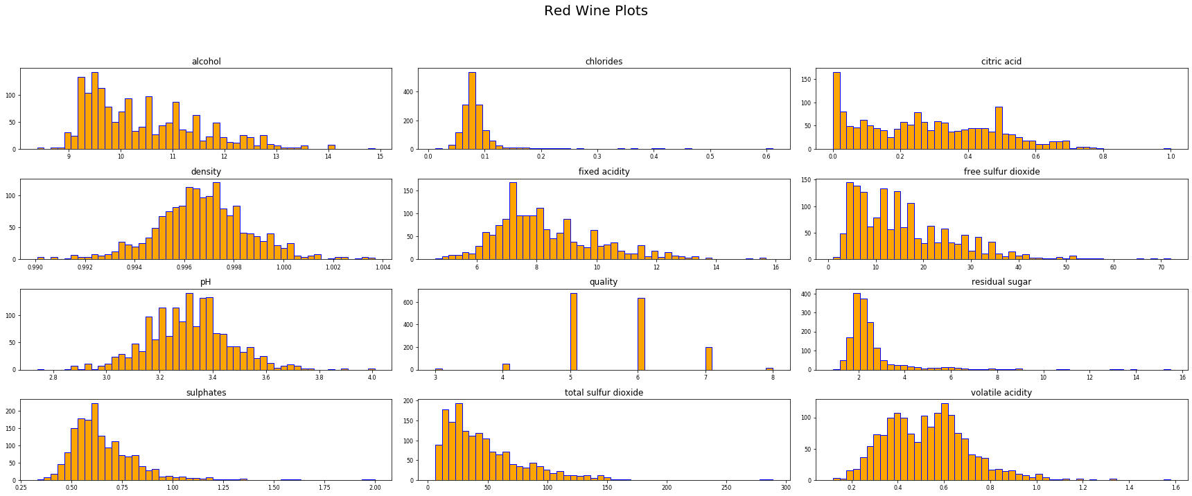
# print out the distribution on each column (variable)
df.hist(bins = 50, edgecolor = 'b', grid = False,
                linewidth = 1.0,
                xlabelsize = 8, ylabelsize = 8,
                figsize = (16, 6), color = 'orange')
plt.tight_layout(rect = (0, 0, 1.5, 1.5))
plt.suptitle('Red Wine Plots', x = 0.75, y = 1.65, fontsize = 20);
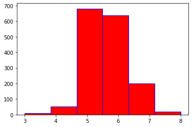
# print out histogram of the quality variable
df['quality'].hist(bins = 6, grid = False, color = 'red', edgecolor = 'b')
<matplotlib.axes._subplots.AxesSubplot at 0x1a1f4fc438>
# print out the correlation matrix (for each column)
df.corr()
| fixed acidity | volatile acidity | citric acid | residual sugar | chlorides | free sulfur dioxide | total sulfur dioxide | density | pH | sulphates | alcohol | quality | |
|---|---|---|---|---|---|---|---|---|---|---|---|---|
| fixed acidity | 1.000000 | -0.256131 | 0.671703 | 0.114777 | 0.093705 | -0.153794 | -0.113181 | 0.668047 | -0.682978 | 0.183006 | -0.061668 | 0.124052 |
| volatile acidity | -0.256131 | 1.000000 | -0.552496 | 0.001918 | 0.061298 | -0.010504 | 0.076470 | 0.022026 | 0.234937 | -0.260987 | -0.202288 | -0.390558 |
| citric acid | 0.671703 | -0.552496 | 1.000000 | 0.143577 | 0.203823 | -0.060978 | 0.035533 | 0.364947 | -0.541904 | 0.312770 | 0.109903 | 0.226373 |
| residual sugar | 0.114777 | 0.001918 | 0.143577 | 1.000000 | 0.055610 | 0.187049 | 0.203028 | 0.355283 | -0.085652 | 0.005527 | 0.042075 | 0.013732 |
| chlorides | 0.093705 | 0.061298 | 0.203823 | 0.055610 | 1.000000 | 0.005562 | 0.047400 | 0.200632 | -0.265026 | 0.371260 | -0.221141 | -0.128907 |
| free sulfur dioxide | -0.153794 | -0.010504 | -0.060978 | 0.187049 | 0.005562 | 1.000000 | 0.667666 | -0.021946 | 0.070377 | 0.051658 | -0.069408 | -0.050656 |
| total sulfur dioxide | -0.113181 | 0.076470 | 0.035533 | 0.203028 | 0.047400 | 0.667666 | 1.000000 | 0.071269 | -0.066495 | 0.042947 | -0.205654 | -0.185100 |
| density | 0.668047 | 0.022026 | 0.364947 | 0.355283 | 0.200632 | -0.021946 | 0.071269 | 1.000000 | -0.341699 | 0.148506 | -0.496180 | -0.174919 |
| pH | -0.682978 | 0.234937 | -0.541904 | -0.085652 | -0.265026 | 0.070377 | -0.066495 | -0.341699 | 1.000000 | -0.196648 | 0.205633 | -0.057731 |
| sulphates | 0.183006 | -0.260987 | 0.312770 | 0.005527 | 0.371260 | 0.051658 | 0.042947 | 0.148506 | -0.196648 | 1.000000 | 0.093595 | 0.251397 |
| alcohol | -0.061668 | -0.202288 | 0.109903 | 0.042075 | -0.221141 | -0.069408 | -0.205654 | -0.496180 | 0.205633 | 0.093595 | 1.000000 | 0.476166 |
| quality | 0.124052 | -0.390558 | 0.226373 | 0.013732 | -0.128907 | -0.050656 | -0.185100 | -0.174919 | -0.057731 | 0.251397 | 0.476166 | 1.000000 |
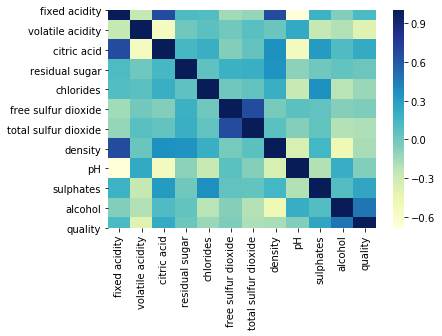
# print out correlation heatmap using 'seaborn' library
sns.heatmap(df.corr(), cmap = "YlGnBu")
<matplotlib.axes._subplots.AxesSubplot at 0x1a1fad1400>
Modeling
Using Linear Regression
# Create a linear regression model:
model = LinearRegression()

# Train ("fit") the model:
model = model.fit(df[ ['fixed acidity', 'volatile acidity', 'citric acid', 'residual sugar', 'chlorides', 'free sulfur dioxide', 'total sulfur dioxide', 'density', 'pH', 'sulphates','alcohol'] ], df['quality'] )
# print out the intercept:
intercept = model.intercept_
intercept
21.965208449448177
# print out the slope (as table):
slope = model.coef_

coeff_df = pd.DataFrame(slope, ['fixed acidity', 'volatile acidity', 'citric acid', 'residual sugar', 'chlorides', 'free sulfur dioxide', 'total sulfur dioxide', 'density', 'pH', 'sulphates','alcohol']  , columns = ['Coefficient'])
coeff_df
| Coefficient | |
|---|---|
| fixed acidity | 0.024991 |
| volatile acidity | -1.083590 |
| citric acid | -0.182564 |
| residual sugar | 0.016331 |
| chlorides | -1.874225 |
| free sulfur dioxide | 0.004361 |
| total sulfur dioxide | -0.003265 |
| density | -17.881164 |
| pH | -0.413653 |
| sulphates | 0.916334 |
| alcohol | 0.276198 |
# create prediction using our model
df["predicted"] = model.predict( df[ ['fixed acidity', 'volatile acidity', 'citric acid', 'residual sugar', 'chlorides', 'free sulfur dioxide', 'total sulfur dioxide', 'density', 'pH', 'sulphates','alcohol'] ] )

df["predicted"] = round(df["predicted"], 0)
df["predicted"]
0       5.0
1       5.0
2       5.0
3       6.0
4       5.0
       ...
1594    6.0
1595    6.0
1596    6.0
1597    5.0
1598    6.0
Name: predicted, Length: 1599, dtype: float64
Results
-
Relationship of
pHandfixed acidity- From the correlation matrix (in EDA section), we can see that
pHandfixed acidityhave the highest correlation with the value of -0.682978.
- From the correlation matrix (in EDA section), we can see that
# Create a scatter plot between 'pH' (x-axis) and 'fixed acidity'(y-axis).
df.plot.scatter(x = 'pH', y = 'fixed acidity')
<matplotlib.axes._subplots.AxesSubplot at 0x1a2009fb00>
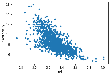
This negative correlation might be obvious and understandable since
- pH is the measure of acidity/basicity with a scale between 0 (very acid) and 14 (very basic) # information taken from chemistry class
- so the more acidic is a solution, pH value will decrease.
- as indicated in the data description, most wines are acidic and have pH values of 3-4 # in this data (lowest = 2.74 and highest = 4.01) obtained from EDA section.
Therefore, we can conclude that there is a causation between pH and fixed acidity.
-
Relationship of
qualityandalcohol- From the correlation matrix (in EDA section), we found out that
alcoholhas the highest correlation with our target or response variablequalitywith a value of 0.476166.
- From the correlation matrix (in EDA section), we found out that
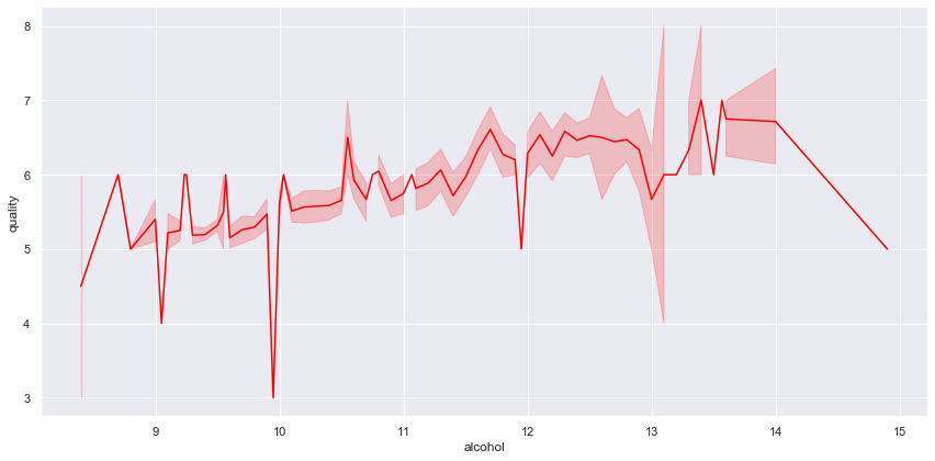
# visualization using 'seaborn' library for scatter plot between 'alcohol' and 'quality'
sns.set()
sns.relplot(data = df, x = 'alcohol', y = 'quality', kind = 'line', height = 6, aspect = 2, color = 'red');
-
The plot above clearly reflects the positive correlation between
qualityandalcohol. Where an increase in the alcohol level (< 14) might result in a better wine quality. -
One important thing to mention is:
- This might not be necessarily true since there are cases where a higher quality level might result in lower wine quality. (in this dataset, for instance, a wine with 9% alcohol level has a lower quality than wine with 8% alcohol level).
- While there is a positive correlation between
qualityandalcoholtheir relationship does not indicate causality.
Discussion
The predictive ability of our model is very low with an accuracy of only 59.16%. This means our model does a really bad job on predicting the wine quality.
- This bad results (predictive power) might be due to:
- Limited predictor variable; in this dataset, we are only given variables that are based on physicochemical tests (lab tests such as alcohol percentage level, pH value, etc.).
- There are many predictor variables that might be more helpful in order to predict the wine quality such as
grape type,wine age,vineyard location, and etc.
# check our model accuracy
(df["predicted"] == df["quality"]).mean()
0.5916197623514696
Solutions and Recommendations:
- Obtain more data (predictor variables and samples) and do another analysis.