Predicting Airbnb house prices
Statistical learning models were applied to Airbnb rental data in order to predict rental prices based on attributes of the rental properties and their associated web listing.
 Image credit: Wynand P
Load Library
Abstract
Most individuals who sleep at their destination would need a “home away from home.” Businesses have always taken care of that. But Airbnb gave the market a fresh and exciting twist. variety of learning techniques were explored and validated, but ultimately the predictive power of the models appears to be limited by the available data. Additional data collection is recommended.
Introduction
When you are away from home for business or pleasure, it is essential that you have a place to relax and rest. 1 The days of calling hotels and comparing rates over the phone are gone for a long time, and using applications to locate, compare, and book hotels or private residences is the way of the present. 2 Airbnb, one of the many options that allow you to rent a personal home or a room in someone else’s house, offering an incredible experience ranging from traditional hotels to luxury mansions. You can read other guest reviews within the app, interact safely with estate owners, and much more. Moreover, you can even list your space and become hospitality entrepreneurs.
3 As Airbnb popularity rises among the public, many including the company itself use the data to find out more about hosts, geographical availability, necessary metrics to make predictions and draw conclusions. Many variables can affect the rental price of an Airbnb listing. However, is it beneficial to predict a rental price? And will be it enough to use only a limited amount of numerical and categorical metrics such as the data provided via Kaggle to estimate the price of rentals?
Statistical learning techniques were applied to several listings from Airbnb in New York during 2019. All variables including name, location, room type, and the number of reviews were used to predict the price of rentals. The results indicate that this prediction is almost impossible to make due to a large amount of error. The importance of predicting the price and statistical limitations suggest the need for further investigation.
Methods
Data
The data was accessed via Kaggle. 4 It contains information on Airbnb listings in New York, NY during 2019 including price, rental attributes, and location. For the purposes of this analysis, the data was restricted to short term (one week or less) rentals in Brooklyn that rent for less than $1000 a night. (Additionally, only rentals that have been reviewed are included.)
airbnb = read_csv(file = "data/AB_NYC_2019.csv")brooklyn = airbnb %>%
filter(minimum_nights <= 7) %>%
filter(neighbourhood_group == "Brooklyn") %>%
filter(number_of_reviews > 0) %>%
filter(price > 0, price < 1000) %>%
na.omit() %>%
select(latitude, longitude, room_type, price, minimum_nights, number_of_reviews,
reviews_per_month, calculated_host_listings_count, availability_365) %>%
mutate(room_type = as.factor(room_type))set.seed(42)
# test-train split
bk_tst_trn_split = initial_split(brooklyn, prop = 0.80)
bk_trn = training(bk_tst_trn_split)
bk_tst = testing(bk_tst_trn_split)
# estimation-validation split
bk_est_val_split = initial_split(bk_trn, prop = 0.80)
bk_est = training(bk_est_val_split)
bk_val = testing(bk_est_val_split)Modeling
In order to predict the price of rentals, three modeling techniques were considered: linear models, k-nearest neighbors models, and decision tree models.
- Linear models with and without log transformed responses were considered. Various subsets of predictors, with and without interaction terms were explored.
- k-nearest neighbors models were trained using all available predictor variables. The choice of k was chosen using a validation set.
- Decision tree models were trained using all available predictors. The choice of the complexity parameter was chosen using a validation set.
fit1 = lm(price ~ ., data = bk_est)
fit2 = step(fit1, direction = "backward")
fit3 = step(lm(price ~ . ^ 2, data = bk_est), direction = "backward")
fit4 = lm(log(price) ~ ., data = bk_est)
fit5 = step(lm(log(price) ~ ., data = bk_est), direction = "backward")
fit6 = step(lm(log(price) ~ . ^ 2, data = bk_est), direction = "backward")
k = 1:100
knn_mods = map(k, ~knnreg(price ~ ., data = bk_est, k = .x))cp = c(1.000, 0.100, 0.010, 0.001, 0)
tree_mods = map(cp, ~rpart(price ~ ., data = bk_est, cp = .x))Evaluation
To evaluate the ability to predict rental prices, the data was split into estimation, validation, and testing sets. Error metrics and graphics are reported using the validation data in the Results section.
calc_rmse = function(actual, predicted) {
  sqrt(mean( (actual - predicted) ^ 2) )
}

calc_rmse_model = function(model, data, response) {
  actual = data[[response]]
  predicted = predict(model, data)
  sqrt(mean((actual - predicted) ^ 2))
}

calc_rmse_log_model = function(model, data, response) {
  actual = data[[response]]
  predicted = exp(predict(model, data))
  sqrt(mean((actual - predicted) ^ 2))
}
Results
rmse_lm1 = calc_rmse(actual = bk_val$price, predicted = predict(fit1, bk_val))
rmse_lm2 = calc_rmse(actual = bk_val$price, predicted = predict(fit2, bk_val))
rmse_lm3 = calc_rmse(actual = bk_val$price, predicted = predict(fit3, bk_val))
rmse_lm4 = calc_rmse_log_model(model = fit4, data = bk_val, response = "price")
rmse_lm5 = calc_rmse_log_model(model = fit5, data = bk_val, response = "price")
rmse_lm6 = calc_rmse_log_model(model = fit6, data = bk_val, response = "price")
lm_val_rmse = c(rmse_lm1, rmse_lm2, rmse_lm3)
log_lm_rmse = c(rmse_lm4, rmse_lm5, rmse_lm6)
knn_preds = map(knn_mods, predict, bk_val)
knn_val_rmse = map_dbl(knn_preds, calc_rmse, actual = bk_val$price)tree_preds = map(tree_mods, predict, bk_val)
tree_val_rmse = map_dbl(tree_preds, calc_rmse, actual = bk_val$price)tibble(
"Model" = c("Linear", "Log Linear", "KNN", "Decision Tree"),
"Tuning" = c("Subset of Interactions", "Subset of Interactions", "k = 44", "cp = 0.001"),
"Validation RMSE" = c(lm_val_rmse[which.min(lm_val_rmse)],
log_lm_rmse[which.min(log_lm_rmse)],
knn_val_rmse[which.min(knn_val_rmse)],
tree_val_rmse[which.min(tree_val_rmse)])
) %>%
kable(digits = 2) %>%
kable_styling("striped", full_width = FALSE)| Model | Tuning | Validation RMSE |
|---|---|---|
| Linear | Subset of Interactions | 66.29 |
| Log Linear | Subset of Interactions | 66.62 |
| KNN | k = 44 | 81.40 |
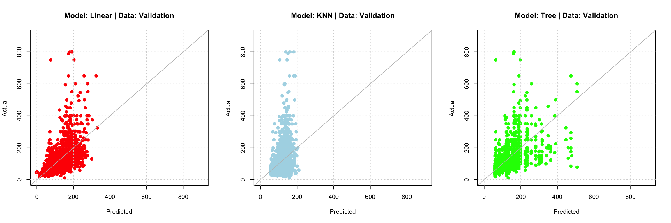
| Decision Tree | cp = 0.001 | 69.02 |
par(mfrow = c(1, 3))

axis_limits = c(0, 900)

plot(predict(fit3, bk_val), bk_val$price,
     xlim = axis_limits, ylim = axis_limits, pch = 19, col = "red",
     xlab = "Predicted", ylab = "Actual",
     main = "Model: Linear | Data: Validation")
abline(a = 0, b = 1, col = "grey")
grid()

plot(predict(knn_mods[[44]], bk_val), bk_val$price,
     xlim = axis_limits, ylim = axis_limits, pch = 19, col = "lightblue",
     xlab = "Predicted", ylab = "Actual",
     main = "Model: KNN | Data: Validation")
abline(a = 0, b = 1, col = "grey")
grid()

plot(predict(tree_mods[[4]], bk_val), bk_val$price,
     xlim = axis_limits, ylim = axis_limits, pch = 19, col = "green",
     xlab = "Predicted", ylab = "Actual",
     main = "Model: Tree | Data: Validation")
abline(a = 0, b = 1, col = "grey")
grid()
Discussion
lm_mod = step(lm(price ~ . ^ 2, data = bk_trn), direction = "backward")
tst_rmse = calc_rmse(actual = bk_tst$price, predicted = predict(lm_mod, bk_tst))
tst_rmse
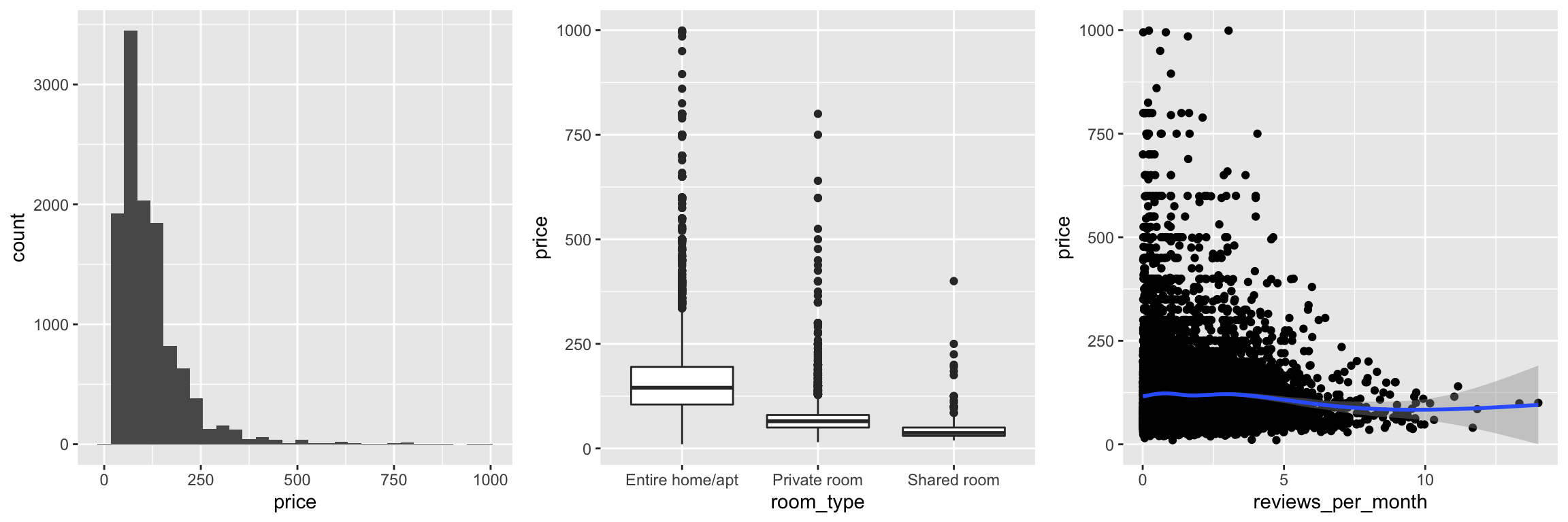
Given the results of assessing model performance on the validation data, the linear model that selects from all available predictors, as well as all two-way interactions using backwards selection and AIC appears to be a reasonable choice. Using the test data, we obtain a RMSE of 72.626 dollars. While the range of prices seen in this data, ranging from roughly 0 to 10,000 dollars, with most observations greater than 50 dollars and less than 200 dollars (from the box plot of room_type versus price), this seems to suggest our model is performing badly at the prediction task.
The provided dataset may be the limiting factor in this analysis. Even with limited domain knowledge, it should be rather clear that the attributes of the rentals are extremely lacking. There are many more variables that might be more helpful in predicting rental prices such as house rules, amenities, cancellation policy, number of positive and ne. It turns out that Airbnb actually releases much more information than is re-hosted on Kaggle. We will use the complete data in our next analysis.
Appendix
Data Dictionary
latitude- latitude coordinates of the listinglongitude- longitude coordinates of the listingroom_type- listing space typeprice- price in dollarsminimum_nights- amount of nights minimumnumber_of_reviews- number of reviewsreviews_per_month- number of reviews per monthcalculated_host_listings_count- amount of listing per hostavailability_365- number of days when listing is available for booking
For additional background on the data, see the data source on Kaggle.
EDA
plot_1 = bk_trn %>%
  ggplot(aes(x = price)) +
  geom_histogram(bins = 30)

plot_2 = bk_trn %>%
  ggplot(aes(x = room_type, y = price, colour = price)) +
  geom_boxplot()

plot_3 = bk_trn %>%
  ggplot(aes(x = reviews_per_month, y = price)) +
  geom_point() + geom_smooth(span = 0.3)

gridExtra::grid.arrange(plot_1, plot_2, plot_3, ncol = 3)
bk_trn %>%
  ggplot(aes(x = longitude, y = latitude, colour = price)) +
  geom_point()